Overview
Background
Use SAXS FrameSlice to improve your calculations by averaging the intensities of different regions of your data after taking multiple images of the same sample. By taking the approach of averaging your data over the different regions of your SAXS profiles you may:
- Determine the limits of radiation-induced aggregation or damage, and adjust your data accordingly, particularly for the Gunier region of your data
- Remove data points from either end of your data
- Improve signal to noise ratios, particularly at the Wide-angle region of your data
Currently, the default Gunier region is defined by a scattering angle of 0.05, and the beginning of the Porod region starts after a scattering angle of 0.25, but these regions may be user adjusted in the "Parameters" section of the app controls.
Usage
- Drag and drop, or upload your files - see general requirements below
- Use slider inputs to average 3 regions of your data
- Download a new averaged file
General Requirements
File Format
The file format for SAXS FrameSlice is based upon the typical processed .dat file type that is produced at the SIBYLS beamline:
- The file extension must be .dat
- The files should not have headers or footers
- The file contents should consist of 3 columns in plain-text using space-delimited values from post-processed image data
- The 3 columns should consist of the 'scattering angle q', 'intensity', and 'errors', respectively
- Values in the columns should be numbers that are either floats or in exponential notation
- The experimental setup should be the same across all files, ie. have the same scattering angles and have the same number of lines of data
Supported Browsers
Uploading Data
File Upload
- Click the white upload box to get a menu dialog to upload your files or...
- Drag and drop your files onto the white upload box
- Chrome, Firefox, Opera, Vivaldi, and Brave users may drag-and-drop a directory folder directly onto the box to upload files
Considerations
- Always wait until the current job is finished (you see the graph) before uploading files to submit another job when using multiple windows from the same browser
- After the files have uploaded and the graph appears, check that all of your files have been processed by looking at the number of files, and their names under the graph
Graph Area

Message at top of graph area
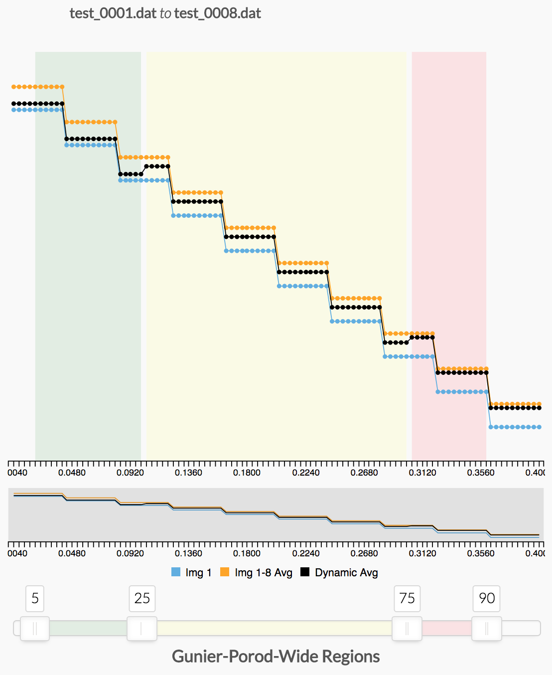
- Displays first and last data file, "test-0001.dat to test-0008.dat", that was processed to generate the data
- If there was an error, a message will appear at this position
Main (upper) graph
- This graph displays three sets of data, in this example the "Line" format has been chosen from the "Chart" controls option:
- Data corresponding to the first processed image (colored blue and labeled "Img 1" in the legend)
- Data corresponding to all images (colored orange and labeled "Img 1-N Avg", where N is the total number of images) - here the angles are all the same (a requirement for this program) - but the intensities are averaged among all files that were uploaded
- Data that you control (colored black and labeled "Dynamic") that represents the eventual output file that will be generated upon hitting the "Download" button
- Upon loading, the "Dynamic" data will overlap with the "Img 1" data until the number of images to include using the data inputs is increased
- The main graph has 3 shaded areas corresponding to different "regions" that may be independently represented by different numbers of image data to include in the average calculation:
- The Gunier region(shaded green)
- The Porod region(shaded yellow)
- The Wide region(shaded red)
- The x-axis of the graph shows the scattering angle
- Zoom and Drag Features:
- Zoom: Hover your pointer over the graph, then use the click-wheel of your mouse to zoom in and out
- Drag: Click the graph and drag to the left of the right
Zoom (lower) graph
- The grey area depicts the relative region of the main upper graph that when zoomed in
- If the chart is in line mode, a corresponding plot of the line is displayed in the zoom graph
- Zoom and Drag Features:
- Drag: When the main upper graph is zoomed in, you may click the lower zoom graph and drag to the left of the right to move the main upper graph
Legend
- Focus and Hide features:
- Focus: To show just one particular graph, hover your pointer over the respective title in legend
- Hide/Unhide: To hide/unhide a graph, click the respective title in the legend
Slider Bar
- When the user input parameters are in "Slider" mode, a slider bar is shown below the graphs
- This slider controls the boundaries of the different regions of the graph again colors correspond to:
- The Gunier region(shaded green)
- The Porod region(shaded yellow)
- The Wide region(shaded red)
- In the example above, data corresponding to lines 5-25 of the input file are selected to represent the Gunier region and will appear in the output when hitting the "Download" button. Likewise, lines 26-75 of the input files will represent the Porod region, and lines 76-90 of the Wide Region. Lines 1-9 and 91-100 will be excluded from the output
- When the parameters are in "Input" mode, the slider bar will disappear and be replaced by input fields in the Control Area
Control Area

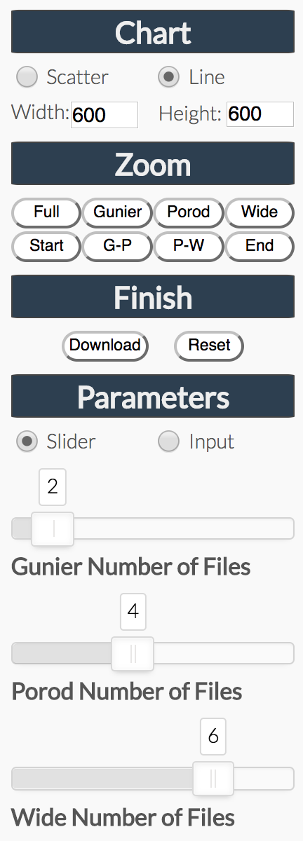
Chart
- Scatter: renders a scatter plot of your data
- Line: renders a scatter plot with lines that connect data points
Zoom
- Full: Zooms out to show the entire data range on the graph (default upon loading)
- Gunier: Zooms in to the Gunier region, as defined by the initial default cutoffs and then by other user-defined controls, plus a few Porod region points
- Porod: Zooms in to the Porod region, as defined by the initial default cutoffs and then by other user-defined controls, plus a few Gunier and Wide region points
- Wide: Zooms in to the Wide region, as defined by the initial default cutoffs and then by other user-defined controls, plus a few Porod region points
- Start: Zooms in to the first data points of your uploaded files
- G-P: Zooms in to the interface between the Gunier and Porod regions of your data
- P-W: Zooms in to the interface between the Porod and Wide regions of your data
- End: Zooms in to the last data points of your uploaded files
Finish
- Download: Downloads the user-adjusted file that represents averaged data across the three regions
- Reset: Reloads the webpage for a new analysis
Parameters
- Slider: Use slider bars to update your dynamic graph:
Here, use the three sliders to determine how many image frames (input files) to include in your "Dynamic" output file for each region. From top to bottom, they represent the following order:
- The Gunier region
- The Porod region
- The Wide region
- Input: Use input boxes or increment arrows to update your dynamic graph
- In "Input" mode, the top three input fields again determine how many image frames (input files) to include in your "Dynamic" output file for each region
- The bottom three input fields below adjust the three regions of the plot, similar to the slider bar that is below the graph when in "Slider" mode, where "Start" and "End" represent the boundaries for each representative section
- Again, the order for the set is Gunier, Porod, Wide
File List

- Shows the actual number of files processed to produce the graph and subsequent output
- Shows the names of the files processed to produce the graph and subsequent output
- The above should be checked in the event it appears that a file did not load properly or if SAXS curves appear strange (unintentionally mixed two or more datasets)
Demo Files
- Click the link to download a .zip file consisting of the test files used in these instructions:
dats-test.zip
- Unzip the directory before uploading files or the folder to the SAXS FrameSlice webapp


